Recursion
In computing, recursion is defining and solving a problem in terms of smaller instances of the same problem.
Factorial
For our first concrete example of recursion, we compute n!, pronounced “n factorial.” Here’s one way to define it:
- n! = 1, if n = 0, and
- n! = n × (n−1) × (n−2) × ⋯ × 1, if n > 0.
Note that the product (n−1) × (n−2) × ⋯ × 1 equals (n−1)!. With this observation, we can recast the definition of n! as
- n! = 1, if n = 0, and
- n! = n × (n−1)!, if n > 0.
That is, if n > 0, we can compute n! by first computing (n−1)! and then multiplying the result by n.
We have defined n! in terms of a “smaller” factorial, namely (n−1)!.
We call the first case (n = 0) the base case, and the second case (n > 0), which uses the value of (n−1)!, is the recursive case.
When writing code, notice that code in the body of the function can
make a call to the function itself. If the actual parameters are
different than in the original call, we might expect different results.
So for example, a recursive factorial function might be
called with the parameter 5. It would then call
factorial(4) to compute the value 24, which it could
multiply by 5 to compute and return 120.
Exercise: recursive factorial
Objective: Write a recursive function, with a base case and a recursive case.
Write the function factorial with no loops, based on the
observation above. You need to handle two cases. First, if the parameter
n has the value 0, then factorial(n) should
simply return 1. Otherwise, the function should compute
factorial(n - 1) and make use of that result to compute and
return the needed value.
Here is a solution. No peeking until you’ve solved it yourself!
How recursion works
Recursive definitions seem inherently circular. Many people have a hard time believing that they can work. Recursion relies on two important properties:
The recursive case breaks the problem into one or more smaller problems of the same kind. It is very important that the new problems be smaller and of the same kind as the original problem.
The method defines one or more base cases, which are solved directly without using recursion. The recursive subdivision described in the first rule must always eventually end up in base cases.
If these two rules are met, recursion works. You work on smaller and smaller problems until you get down to a base case. It may take you a little while to get comfortable with recursion, however. In the meantime, let’s see what really happens in the computer. Thinking about what goes on inside the computer while trying to write complicated recursive functions is a good way to get a headache. Think in terms of the two rules above, and have faith that if you follow them that the program will work.
Stack frames and the call stack
Before looking too closely at recursion yet, let’s look at how function calls work. At any instant in time, the program counter points at some location in the code: the line number of the code that is being executed and where Python is in that line.
While a function is running, Python needs to store some information about the local variables for that function. The values of the local variables are stored in a piece of memory called a frame. When the function returns, those local variables are not longer in scope, and can be destroyed; the frame associated with the function is destroyed.
What if one function, functionA calls another,
functionC? Well, the code in functionC should
not have access to the local variables of functionA, but
when functionC returns back to functionA, then
the local variables of functionA will once again be
needed.
So, while functionC is running, Python needs to have two
frames: one for functionA, and one for
functionC, but only the frame for functionC is
active.
These frames are stored in a structure called the call stack. The currently running function has a frame that is accessible, at the top of the stack. Below that in the stack is the frame for the suspended function that called the currently running function.
Step through the following example, in call_stack.py. Notice that the “top” frame is drawn on the bottom of the page, because it is easier to draw that way. As each function is called, another frame is added to the stack. When a function returns, its frame is popped from the stack and destroyed, since the local variables are no longer needed once the function terminates.
We can look at the “lifetime” of a function chronologically:
- The function is called, and it starts running.
- Later, the function might call another function. If so, the function suspends while the other function executes.
- Eventually, the original function resumes execution when the function it called finishes.
- Finally, the function terminates when Python reaches a return statement or the end of the function body.
As a function executes, space is created in memory for any local variables. If a second function is called from within the first function, the local variables of the first function are not destroyed, but are inaccessible to the second function. This makes sense, right? Local variables of the first function need to still exist after the second function finishes, and the first function is only suspended. Local variables of the first function will not be destroyed until the first function itself terminates.
At any instant, just one function is actively running, but there may be many suspended functions, these being the function that directly called the current function and the function that called that function, etc. For both the currently running function and any suspended functions, Python needs to store
- where to return the program counter to after the function terminates, and
- the values of any parameters and other local variables.
The call stack in recursive code
Now that we see how the call stack is organized, let’s examine what
happens when we call factorial(3). After several recursive
calls, we hit the base case, and the call stack looks like this:

I wrote in the return value of the call factorial(0), 1,
to the right of the stack frame. After factorial(0)
terminates and its frame is popped, factorial(1) multiplies
n by 1 and returns that value (1, since
n = 1) to factorial(2). Then
factorial(2) mutliplies the value returned from
factorial(1) by 2 and returns 2. You should walk through
the code, crossing off stack frames as they are popped, and writing the
value each function call returns next to its stack frame.
Notice that although the factorial function has a local
variable (actually, a formal parameter, but you know that each formal
parameter is also a local variable, right?) named n,
each stack frame has its own version of this variable.
Again, different variables with the same name. Although they are in the
same function, they are in different calls of this function.
Every time you call a function, a new stack frame is created for the
call, and each stack frame contains a slot for all the local variables
(including formal parameters) of that function.
Infinite recursion
One mistake that you might make when programming recursive methods is
to fail to ensure that you hit the base case. Suppose that you called
factorial(-1). It would call factorial(-2)
which would call factorial(-3), and so on until you got the
error message
RuntimeError: maximum recursion depth exceeded. We didn’t
make sure to hit the base case eventually.
Another mistake is not making the subproblems smaller. It is true that n! = (n+1)!/(n+1). Try editing your recursive factorial program to change the recursive call to:
return factorial(n + 1) / (n + 1)The call factorial(n) makes the call
factorial(n + 1), which makes the call
factorial(n + 2), and so on. In either case, each call
causes a new stack frame to be pushed, and eventually you run out of
memory, resulting once again in the dreaded
RuntimeError: maximum recursion depth exceeded message.
Side note: Slicing lists and strings
We’re going to reverse a string recursively in the next section. Before we do that, here are a few Python tricks that are good to know for dealing with lists and strings.
Negative indices count items from the end.
If you want a substring of a string (or a sublist of a list), you can “slice” it by using a colon inside the square brackets:
Notice that the substring or sublist starts at the index before the colon and goes up to but not including the index after the colon.
You can get the end of a string even more easily by omitting the number after the colon:
Another side note: Since you cannot change the value of a string, you cannot use the slice operator to insert characters into a string. (You actually can insert values into a list this way, but we will not use that trick any time soon.)
Reversing a string
It is useful to be able to reverse the characters in a string, and
recursion gives us an easy way to do so. (Iteration does also, but we’re
focusing on recursion here.) Let’s define the tail of
the string as all characters except for the first one. For example, in
the string ward, the tail is ard.
Then we can reverse a string as follows:
- Remove the first character of the string, and remember it.
- What’s left is the tail. Recursively reverse the tail.
- Concatenate the remembered first character onto the end of the reversed tail.
For example, when we reverse ward, we reverse the tail
ard, getting dra. Concatenating the leading
w to the end gives us draw.
Because the tail is shorter than the original string, we are dealing with a smaller problem of the same type.
What is the base case? A string with no characters is its own reverse, and we can return it without a recursive call.
Exercise: recursive reverse
Objective: Write a recursive function, based on a description of the base case and recursive case.
Write a recursive function to reverse a string. The base case occurs
when the string is the empty string "". The recursive case
involves appending the first character of the string to the reversed
tail of the string, where the tail is the string without the first
character.
Here is a solution. No peeking until you’ve solved it yourself!
Recommended exercise: Draw the call stack and write
down the output while tracing through the reverse function
line-by-line.
Fibonacci numbers
The nth Fibonacci number, fib(n), is defined as follows:
- fib(1) = fib(2) = 1, and
- fib(n) = fib(n−1) + fib(n−2), if n > 2.
Here’s a table with the first eight Fibonacci numbers:
| n: | 1 | 2 | 3 | 4 | 5 | 6 | 7 | 8 |
|---|---|---|---|---|---|---|---|---|
| fib(n): | 1 | 1 | 2 | 3 | 5 | 8 | 13 | 21 |
Expressed recursively:
- Base cases: n = 1 and n = 2.
- Recursive case: We know how to compute fib(n−1) and fib(n−2). Use them to compute fib(n).
Here is some recursive code to compute the n-th Fibonacci number:
This program uses two recursive calls. We need to keep track of exactly where each call was made. Are we returning to the first or to the second recursive call? Keeping track of where we are in the program is hard for people to do without making mistakes, but computers are quite good at it. They don’t get distracted.
A helpful way to visualize what happens in recursive programs is a
recursion tree. A recursion tree has
nodes connected by branches, or
links. Here’s a recursion tree for computing
fib(3):

The way to interpret a recursion tree like this one is that we label each node with the value of n at a call, and each link denotes a call. In this case, the call for n = 3 ends up making two calls, one for n = 2 and one for n = 1.
For our fib method, whenever the call is for a value
n that is greater than 2, fib will make two
recursive calls, one for n − 1
and one for n − 2.
For n = 6, for example, we get the following recursion tree:
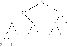
In computer science, we draw trees with the root at the top; for this tree, the root is labeled 6. The nodes on the bottom are leaf nodes, or leaves, because if we drew the tree with the root at the bottom, they would look like leaves of the tree.
Notice that we repeat a lot of work. For example, to compute
fib(6), we call both fib(5) and
fib(4). But we also call fib(4) in computing
fib(5). Each call to fib(4) will return the
same result. Yet we end up making separate calls to fib(4),
repeating the work each time.
Notice also that there are 8 leaf nodes. Each leaf node corresponds
to a call that is a base case. Each base case returns 1, thereby
contributing 1 to the eventual result. So it should be no surprise that
there are 8 leaf nodes, when the call fib(6) returns 8.
If fib(n) equals x, then this recursive program ends up in the base case x separate times. In other words, it sums up the value 1 a total of x times. The problem is that the value of fib(n) is exponential in n. (In particular, it is $((1 + \sqrt 5 ) / 2)^n / \sqrt 5$, rounded to the nearest integer.) So, the number of times we get down to a base case is exponential in n, meaning that it gets very large very quickly.
This recursive Fibonacci program is easy to write, but there are far more efficient ways to compute Fibonacci numbers. (In fact, I just told you one: compute the value of a particular expression and round it.)
Exercise: recursive Fibonacci call order
Objective: Trace the execution of a recursive function, listing the order in which function calls are made.
The recursion tree shows which function calls are made, but does not
give the order in which function calls are made. In the text box, write
out the order of function calls for fib(5). The first two
calls are already written. Indent each line of text by a number of tabs
equal to the depth in the recursion tree.
Here is a solution. No peeking until you’ve solved it yourself!
The Towers of Hanoi
Our next example of recursion solves a puzzle called The Towers of Hanoi.
The Towers of Hanoi puzzle has three pegs, numbered 1, 2, and 3. On peg 1 are n disks, in increasing order by size, with the smallest disk (disk 1) on top and the largest disk (disk n) on the bottom. The object is to move all disks from peg 1 to peg 2, obeying two rules:
- Only one disk may be moved at a time. The other disks must be resting on one of the three pegs. These rules imply that only the top disk on a peg may be moved.
- No disk may ever rest on a smaller disk.
The Towers of Hanoi puzzle is being solved, even now, by monks in the high, inaccessible reaches of Tibet. They use 64 disks, and they believe that when they have completed moving all 64 disks from peg 1 to peg 2, the world will come to an end.
If you were to write a recursive function to solve the problem, your function might have the header
solve_hanoi(n, start_peg, end_peg)This function moves all disks numbered 1 through n from peg
start_peg to peg end_peg. It uses the
remaining peg as a spare.
How do you solve this problem? Let’s start with a really easy case: n equals 1. There is only disk 1, and we can just move it from peg 1 to peg 2. Notice that there is nothing special about pegs 1 and 2. We could just as easily move disk 1 from peg 1 to peg 3, or from peg 3 to peg 2, etc.
Now let’s look at what happens when n equals 2. We move disk 1 from peg 1 to the spare peg, which is peg 3. Now disk 2 is exposed, and we can move it from peg 1 to peg 2. All that remains is to move disk 1 from peg 3 to peg 2. Again, there is nothing special about pegs 1 and 2. We could just as easily have moved disks 1 and 2 from peg 1 to peg 3 (move disk 1 from peg 1 to peg 2, move disk 2 from peg 1 to peg 3, move disk 1 from peg 2 to peg 3), or from peg 3 to peg 2 (move disk 1 from peg 3 to peg 1, move disk 2 from peg 3 to peg 2, move disk 1 from peg 1 to peg 3), etc.
How about when n equals 3? We would like to get disk 3 exposed on peg 1 and have no disks on peg 2. In other words, we would like to move disks 1 and 2 from peg 1 to peg 3. But that’s a subproblem that we just said we know how to solve! So we do it, and then we can move disk 3 from peg 1 to peg 2. It remains to move disks 1 and 2 from peg 3 to peg 2. Again, we know how to solve this subproblem.
In general:
- Base case: n equals 1. We just move disk 1 from
start_pegtoend_peg. - Recursive case: n is at least 2. Assume that we
already know how to move disks 1 through n–1 from any peg to
any other peg.
- Determine which peg is the spare peg. Trick: We know that the pegs are numbered 1, 2, and 3. Since we know the numbers of two of them, then the remaining peg must be the sum 1+2+3 (by advanced mathematics, you can show that this sum is 6), minus the two pegs whose numbers we know.
- Solve the subproblem of moving disks 1 through n − 1 from the start peg to the spare peg. Now the end peg is empty, and the start peg holds only disk n.
- Move disk n from the start peg to the end peg.
- Solve the subproblem of moving disks 1 through n − 1 from the spare peg to the end peg.
It takes 2n − 1 moves to solve the Towers of Hanoi. Back to the monks. They’re using n = 64 disks, and so they will need to move a disk 264 − 1 times. These monks are nimble and strong. They can move one disk every second, night and day. How long is 264 − 1 seconds? Using the rough estimate of 365.25 days per year (we’re not accounting for skipping the leap year once every 400 years), that comes to 584,542,046,090.6263 years. That’s 584+ billion years. The sun has only about another five to seven billion years left before it goes all supernova on us. So, yes, the world will end, but no matter how tenacious the monks may be, it will happen long before they can get all 64 disks onto peg 2.
Exercise: towers of Hanoi
Objective: Write a solution to a recursion problem that combines the results of two recursive calls to solve each level of recursion.
The hanoi module provided for this exercise has a
function move moves a disc from one peg to another peg. For
example, move(1, 2) moves a disc from the first peg to the
second peg; pegs are numbered from one to three.
Write the body of the recursive function solve_hanoi. As
an example of how it should work, solve_hanoi(5, 1, 2)
would move 5 discs from peg 1 to peg 2.
solve_hanoi(3, 3, 1) would move 3 discs from peg 3 to peg
1.
Here are some hints:
- Don’t forget the base case. Write and test this first.
- For the recursive case, compute the spare peg by subtracting the sum
of the other two pegs from 6.
- For the recursive case, move some pegs to the spare peg. Then move
one peg to
to_peg. Then move some pegs from the spare peg toto_peg.
Here is a solution. No peeking until you’ve solved it yourself!
Graphics and recursion
If we want to draw something that is similar to itself, recursion can be a good way to go about it. A branch of a tree looks a bit like a little tree, for example, and a piece of a snowflake may itself look like a little snowflake.
Sierpinsky Gasket
Here is a fun example, the Sierpinsky Gasket. The base case is that a Sierpinksy gasket of size one is drawn as a single pixel. The recursive case dives the region up into four quadrants, and draws gaskets in all but the bottom left quadrant.
The Wheel
Here’s a longer example. Wheels within wheels! See if you can figure out how it works.