Linked lists
For the next few lectures, we will be looking at how to implement and use different types of data structures. We have already seen an example of a data structure: a Python list. In general, data structures:
- provide a place to efficiently store and retrieve items of information;
- express some relationship between items; and
- allow algorithms to find, reorder, or apply operations to items in the data structure, using the implied relationship between the items.
Does the Python list provide a place to store and retrieve items?
Yes; for example, we might have a list of numbers, strings, or addresses
of Body objects. What relationship can the list express
among items? The items are in some order implied by the indices
of items in the list. For example, we say that the fourth item follows
the third item in the list, and it precedes the fifth item. We have seen
algorithms that reorder the list (changing the relationship between
items), find items in the list, or just apply operations to each item in
the list (for example, compute the acclerations and velocities of all
planets in a list of planets).
Linked lists are a type of data structure that you have not seen yet in this course. Unlike Python lists, linked lists are not built in to Python, and we will have to implement them ourselves.
Linked lists provide many of the same features that Python lists do:
- Linked lists contain an ordered sequence of items.
- You can append, insert, or delete items from a linked list.
- You can traverse a linked list, applying a function to each item in the list in order.
For many purposes, Python lists are a good choice for containing several items in sequential order. Because Python lists are built into the language, they have been optimized for speed, and the time costs for accessing, deleting, changing, or adding an item have small constant factors associated with them. Since we will write our own linked lists, Python has to interpret the code we write, which will take some time. Nevertheless, for sufficiently large numbers of items, linked lists may provide some advantages for some operations.
Time costs of operations on Python lists
Let’s look at how Python lists actually work. The items in a Python list are stored in order in memory. Consider a list of 4-byte integers. The 0th item in the list is stored at some address, let’s say 7080. Then the first item would be stored at 7084. The second item would be at 7088, and so on. The ith item would be at address 7088 + 4i.
Running time of inserting an item into a Python list
Let’s say you have a Python list with 20 items. You would like to
maintain the order of the items, and you would like to insert a new item
as the first item of the list. You can do this with the
insert method of lists, like this:
The new item will be at index 0. Notice that the item previously at index 0 has to move to index 1, the item previously at index 1 has to move to index 2, and so forth. With some cleverness, you might realize that the best way to do this operation would be to start at the end of the list and move each item one position to the right (does this idea remind you of insertion sort?), but no amount of cleverness will save you from having to loop over each item in the list and moving it.
Inserting into the beginning of the list is the worst case, since all other items have to be moved to the right; inserting at the end of the list is much cheaper. So the worst-case running time for insertion into an n-item Python list is Θ(n).
Time cost of appending to a list: amortized running time
You might think that appending to the list (inserting at the end) would have running time Θ(1), since items do not have to be copied. As one of my favorite faux titles for a country song goes, “Purt near but not plumb.” That is, it’s almost true. Here’s why it is not entirely true. The list is stored in one sequential area of memory. What happens if you try to make the list longer, and there is something stored in memory just after the list? In this case, Python requests a new, larger amount of memory; the computer finds a new location, and relocates the list to that new location by copying the entire list. If the list has n items, then copying the list takes Θ(n) time, and so in the worst case (the situation where the list has to be moved), appending to the list takes Θ(n) time. That is, of course, a lot worse than the Θ(1) time that you might have expected.
But the designers of Python used a very clever idea to make sure that this worst-case running time for appending to a list occurs infrequently. We’ve just seen that when Python appends to an existing list and runs out of space, it has to request a new chunk of memory, where it will move the list. Let’s say the list length is n. But instead of requesting enough space for a list of size n + 1, Python arranges to have room for the new list to grow, and it requests space for a list of size 2n. Overallocating in this way might seem as though it wastes a lot of space—Python allocates up to twice the amount of memory that the list really needs. But the advantage is that if you append items to the list over and over again, the list is moved infrequently.
Let’s say you add 128 items to a list in order, starting with a list of size 1. As you append items to the list, Python will increase the memory allocated to the list. At first, there is memory for 1 item. Then for 2 items. When that space fills up, Python allocates a list with space for 4 items. When that fills up, space for 8. Then 16, 32, 64, and finally, 128. Let’s see what happens as we increase the list size from 64 to 129.
Imagine that it costs 1 dollar to append an item to a list if Python does not have to reallocate space and copy all the items, and that it costs 1 dollar per item to copy items when the list is copied to a new location. When we append an item to the list, let’s charge not 1 dollar, but 3 dollars. Of the 3 dollars, we’ll use 1 dollar to pay for the append operation, and we’ll squirrel away the other 2 dollars in a bank account; we’ll spend this 2 dollars later.
Our list has 64 items, and now let’s append another 64 items. We’re charged 64 × 3 dollars for these append operations, with 64 dollars going toward paying for the appends and the remaining 128 dollars going into the bank. Now we add the 129th item. Before appending this item, we have to copy all 128 of the previous items into reallocated space. But we have 128 dollars already in the bank to pay for it! So we spend the 128 dollars to copy the 128 items, and then we can append the 129th item, paying 1 dollar for the append operation and banking the other 2 dollars.
The key idea here is that the list size doubles. Each item pays 1 dollar for its own append, and it pre-pays 1 dollar for itself to be copied one time and 1 dollar for some previously appended item to be copied one time. Since we pay a constant amount, 3 dollars, for each item we can think of the average time per append being constant, or Θ(1).
We call this sort of analysis an amortized running time analysis, because the possibly expensive cost of adding one item to the list is offset by frequently adding items to the end of the list cheaply. We can “amortize” the cost over several append operations, and show that the behavior of the append operation is pretty good over the long run.
Time cost of deleting an item from a list
If you would like to maintain the order of the list and also delete
an item, then the worst-case cost for an n-item list is Θ(n), since all items
following the deleted item have to be moved up by one position in the
list. You can delete items from a list using the special built-in
operator del in Python:
del my_list[3]Deleting from the end is a special case that is not expensive, since
no items in the list have to be moved; deleting from the end has time
cost Θ(1). We call deleting
from the end popping, and there is a special
pop method on lists that removes from the end, returning
the item that was removed.
Time cost of finding an item in a list
If the list is unsorted, then it takes O(n) time to find an item in an n-item list, by using linear search. Similarly, finding the smallest or largest item in an unsorted list takes Θ(n) time. (It’s Θ(n) and not just O(n) because you don’t know whether you have the smallest or largest item until you’ve seen them all.)
Tricks: Unordered lists (sets)
A list maintains items in order. But sometimes you do not care about
the order of items in the list. You can use this observation to
sometimes insert or remove items without incurring a Θ(n) running time. If the
order doesn’t matter, just insert by appending. When you delete an item
from the list, instead of shifting all the items that follow the deleted
item, you can fill the hole left by the deleted item by moving in the
item that’s at the end of the list. In Python, however, you should
probably more properly use the built-in set data structure
to store items for which you do not care about the order. We will not
discuss the set data structure further at this time, but
you are welcome to look it up in the Python documentation.
Linked lists
Linked lists, like Python lists, contain items in some order, but the implementation of linked lists will be very different from that of Python lists. There are two reasons we will implement our own linked lists:
Certain operations for linked lists are efficient in terms of time. For example, inserting an item into the list costs Θ(1) time, no matter where in the list the item is inserted—much better than the Θ(n) time for inserting into an n-item Python list. For large enough linked lists, in a situation where insertion anywhere in the list is frequent, a linked list might be the better choice, despite the smaller constant factor for Python lists.
The approach we will use to create the linked list is an example that we will build on to form more complex data structures, trees and graphs, that express more interesting relationships between data than the simple sequential list structure.
Nodes in the list
Conceptually, we will create a linked list by making lots of objects
called nodes. Each Node object will
contain an item: the data in the list. The Node objects
themselves could be anywhere in memory, and will typically not
be stored sequentially, or in any other particular order, in memory.
How, then, can we tell which item in the list is first, which is
second, and what the order of items is? Each Node object
will contain an instance variable that has the address of the next
Node object in the linked list.
Let’s look at an example of how this might work. (I should emphasize that this is not yet a good implementation of a linked list. I just want to show you how nodes work.) Here’s a picture of a linked list holding the names of three states, in order: Maine, Idaho, and Utah:
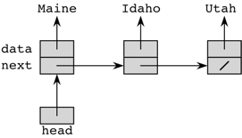
The arrows indicate references. The slash in the next
instance variable of the last Node object (the one whose
data is Utah) is how I indicate the value None
in a picture.
Here’s some simple code. Although we usually put a class in its own
file, I didn’t put the Node class in its own node.py file
because I wanted to keep this example short and in one place.
When we printed the list, we created a new, temporary variable
node that initially has the address of the first
Node object in the linked list. We use that address to find
the data to print (Maine), and then we update
node to hold the address of the next item. We print its
data (Idaho) and update node again to hold the
address of the next item. We print its data (Utah), and
update node once again. Now, node equals
None, and we drop out of the while-loop.
Exercise: linked list of even numbers
Objective: Write a program that adds several items to a linked list using a loop.
Write a program that adds all of the even numbers from 0 to 100 to a
linked list, and then prints out all of the items in the list. To save
some typing, a simple Node class is provided, as is the
code to print the list. You will need to do several things to create the
linked list.
- Create a first node; call it
head. - Create a variable
currentthat will point to the node we are currently working on. - For each data item, create a node and store a reference to it in an
instance variable of
current. Then updatecurrentto point to the next node in the list we are building.
Here is a solution. Do not look at it until you have completed the exercise yourself.
Exercise: needle in a linked list
Objective: write a method that implements an algorithm on a simple linked list.
Write a method find of the Node class that
is passed a data item as parameter, and returns a reference to the first
node in the linked list containing that item, or `None’ if the item is
not found. (Use a loop to search for the item.)
Here is a solution. Do not look at it until you have completed the exercise yourself.
Exercise: recursive find
Objective: write a method that implements a recursive algorithm on a simple linked list.
Write a method find of the Node class that
is passed a data item as parameter, and returns a reference to the first
node in the linked list containing that item, or `None’ if the item is
not found. This time, write the method to search for the item
recursively. Specifically, one of the following three things is true: we
have found the item in the current node, we are at the end of the list,
or the node is in the linked list starting at the next item. Your
solution should not use any for-loops or while-loops.
Here is a solution. Do not look at it until you have completed the exercise yourself.
Circular, doubly linked list with a sentinel
We did some things manually in the above example. It would be nice to have a class for a linked list that stored the address of the first node, and that also provided methods for inserting into, deleting from, appending to, and finding items in the list.
Our previous model for a linked list, in which only the address of the next node is stored in any node, has some annoying special cases. We will therefore start with a slightly different implementation that has a few convenient features that at first blush might seem more complicated, but actually simplifies the implementation of certain methods, and even improves the running time of certain methods.
The list will be doubly linked: each node will contain a reference to the previous node in the chain (in a
previnstance variable) as well as a reference to the next node. This structure not only makes it easy to iterate backward through the list, but it makes other, more common, operations easy, too.The list will have a sentinel node, instead of a reference to a first node. This sentinel node is a special node that acts as the 0th node in the linked list. No data is stored in this special node; it’s there just as a placeholder in the list.
The list will be circular. The last node containing data will hold in its
nextinstance variable the address of the sentinel node, and the sentinel node’sprevinstance variable will hold the address of the last node.
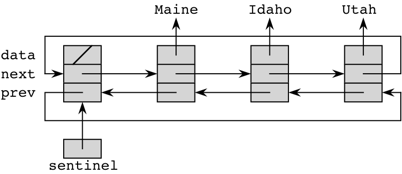
We call this structure a circular, doubly linked list with a sentinel. Quite a mouthful, indeed. Practice saying it fast.
A circular, doubly linked list with a sentinel has the property that every node references a next node and a previous node. Always. This uniform way of treating nodes turns out to be quite convenient, because as we write methods to insert or delete nodes into the list, we don’t have to worry about special cases that would arise if the last node didn’t have a next node, and the first node didn’t have a previous node, but all interior nodes had both.
Here is a picture of a circular, doubly linked list with a sentinel representing the same list as before:
We create a class, Sentinel_DLL, to implement a
circular, doubly linked list with sentinel in sentinel_DLL.py:
Creating an empty list:
__init__
A Sentinel_DLL object has just one instance variable:
sentinel. This instance variable is a reference to a
Node object. I defined the Node class in the
sentinel_DLL.py file, rather than defining it in its own file, because
it’s meant only to be part of a circular, doubly linked list with a
sentinel.
In order for the list to be circular, both the next and
prev instance variables of the sentinel node must contain
the address of the sentinel itself. Here’s what an empty list looks
like:
![]()
It can at first be intimidating to see a line with as many dot operators in it as
self.sentinel.next = self.sentinelJust work left to right for each variable. self is the
address of a sentinel_DLL object.
self.sentinel is the value of the sentinel
instance variable in the sentinel_DLL object. We know that
this value contains the address of some Node object. So
self.sentinel.next is the next instance
variable of the sentinel node in the sentinel_DLL object.
That’s what we’re assigning to. The value we’re assigning is
self.sentinel, the address of the sentinel node.
Finding the first node
The first_node method just returns a reference to the
first node in the list, or None if the list contains just
the sentinel. The first node is always the one after the sentinel. If
the node just after the sentinel is the sentinel itself, then the list
contains just the sentinel, and the method returns None.
Otherwise, the method returns a reference to the first node.
Inserting a new node into a list
To insert a new node into the list, we need to know which node we’re
inserting it after. The parameter x is a reference to that
node. The parameter data gives the data that we’re
inserting.
First, the method creates a new Node object, referenced
by y, to hold the data that we want to add to the list. Now
we need to “splice” the new node into the list, just as you can splice a
new section into a piece of rope or magnetic tape. In order to splice in
the new node, we need to do a few things:
- Make the links in the new node refer to the previous and next nodes in the list.
- Make the
nextlink from the node that will precede the new node refer to the new node. - Make the
prevlink from the node that will follow the new node refer to the new node.
We have to be a little careful about the order in which we do these
operations. Let’s name the nodes for convenience. We already have
x referencing the node that the new node, referenced by
y, goes after. Let z reference the next node
after x before we insert y, so that
y is supposed to go between x and
z. If we clobber the value of the next
instance variable of x too soon, we won’t have a way to get
the address of z, which we will need.
It’s good to be comfortable with the dot notation used so heavily in
the code, but it may help you to draw a picture. Here’s the same method
as above, but with a temporary variable introduced for
z:
    # Insert a new node with data after node x.
    def insert_after(self, x, data):
        y = Node(data)   # make a new Node object.
        z = x.next       # y goes between x and z

        # Fix up the links in the new node.
        y.prev = x
        y.next = z

        # The new node follows x.
        x.next = y

        # And it's the previous node of z.
        z.prev = y
Iterating over a list
The __str__ method shows an example of how to iterate
over a list. The first node in the list is the node after the sentinel.
We loop over nodes, letting x reference each node in the
list, until returning to the sentinel again (recall that the list is
circular). To get to the next node in the list, we use the line
x = x.next.
One other interesting thing about the __str__ method is
that I wrote it to produce the same string as you’d see if the linked
list were a regular Python list. When Python prints a list, it puts
single quotes around all strings in the list. So I have a check to see
whether x.data is a string, and if it is, I add in the
single quotes. I use the built-in Python function type,
which returns the type of its argument. (You can play with this function
in the Python interpreter, IDLE.)
Deleting from a list
The delete method takes a node x and
deletes it from the list. It’s deceptively simple in how it splices the
node out, by just making its next and previous nodes reference each
other. Just we did for insertion, let’s rewrite the delete
method, but with y referencing x’s previous
node and z referencing x’s next node:
    # Delete node x from the list.
    def delete(self, x):
        # Splice out node x by making its next and previous
        # reference each other.
        y = x.prev
        z = x.next
        y.next = z
        z.prev = y
Searching a list
The find method searches the linked list for a node with
a given data value, returning a reference to the first node that has the
value, or None if no nodes have the value. It uses linear
search, but in a linked list.
There’s a cute trick that I’ve incorporated into my implementation of
find. If you go back to the linear search code that we saw before,
you’ll notice that each loop iteration makes two tests: one to check
that we haven’t reached the end of the list and one to see whether the
list item matches what we’re searching for:
def linear_search(the_list, key):
    index = 0
    while index < len(the_list):
        if key == the_list[index]:
            return index
        else:
            index += 1

    return None
Suppose that you knew you’d find the item in the list. Then you wouldn’t have to check for reaching the end of the list, right? So let’s put the value we’re looking for into the linked list, but in a special place that tells us if that’s where we find it, then the only reason we found it was because we looked everywhere else before finding it in that special place.
Gosh, if only we had an extra node in the list that didn’t contain
any data and was at the end of the list. We do: the sentinel. So we put
the value we’re looking for in the sentinel’s data instance
variable, start at the first node after the sentinel, and loop until we
see a match. If the match was not in the sentinel, then we
found the value in the list. If the match was in the sentinel,
the the value wasn’t really in the list; we found it only because we got
all the way back to the sentinel. In either case, we put
None back into the sentinel’s data instance
variable because, well, my mother told me to.
Appending to the list
The only other method in my Sentinel_DLL class is
append. Not surprisingly, it finds the last node in the
list and then calls insert_after for that node. How to find
the last node in the list? It’s just the sentinel’s previous node.
Running times of the linked-list operations
What are the worst-case running times of the operations for a circular, doubly linked list with a sentinel? Let’s assume that the list has n items (n + 1 nodes, including the sentinel, but of course the + 1 won’t matter when we use asymptotic notation).
The __init__, first_node,
insert_after, append, and delete
methods each take Θ(1) time,
since they each look at only a constant number of nodes.
The __str__ method takes Θ(n) time, since it has to
visit every node once.
The time taken by the find method depends on how far
down the linked list it has to go. In the worst case, the value is not
present, and find has to examine every node once, for a
worst-case running time of Θ(n).
Testing the linked list operations
You can test the linked list operations by writing your own driver. I have a pretty minimal driver here: