Graphs
We often need to model entities that have connections between them. For example, we might want to know whether two people are friends. If we can identify a group of people all of whom are friends with each other that might tell us something about these people; for example, they might all be members of the same Greek house, or that they might constitute a terrorist cell.
For another example of entities with connections, think of a road map. Each intersection is an entity, and a connection is a road going between two intersections.
Here’s another example. When you get dressed, there are some articles of clothing that you must put on before other articles, such as socks before shoes. But there are also some articles for which the order that you don them does not matter, such as socks and a shirt. So we can say that there’s a connection between two articles of clothing if you have to put on one before the other.
Sometimes we need to know more than just that there’s a connection; there’s some quantitative aspect of the connection that’s important. For a road map, we might care not only that a road connects two intersections, but also about the length of the road. For another example, we might want to know, for any pair of world currencies, the exchange rate from one to the other.
Many years ago, mathematicians devised a nice way to model situations with many entities and relationships between pairs of entities: a graph. A graph consists of vertices (singular: vertex) connected by edges. Each edge connects one vertex to some other vertex. A vertex may have edges to zero, one, or many other vertices. Think of each vertex as representing an entity and each edge as a connection.
Here’s a simple graph with 9 vertices and 11 edges:
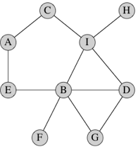
Each vertex in this particular graph is labeled by a letter, though in general we can label vertices however we like, including with no label at all. Just to take an example, vertex A has two edges: one to vertex C and one to vertex E.
In some situations, we want directed edges, where we care about the edge going from one vertex to another vertex. Directed edges work well in the example about getting dressed, where an edge from a vertex for article X to a vertex for article Y indicates that you have to don X before Y. In other situations, such as the graph drawn above, the edges are undirected. Because the friendship relation is symmetric, if we consider a graph in which vertices represent people and an edge between persons X and Y indicates that X and Y are friends, this graph would have undirected edges. A graph with undirected edges is an undirected graph, and a graph with directed edges is a directed graph. We can always emulate an undirected edge between vertices x and y with directed edges from x to y and from y to x.
When we put a numeric value on an edge, say to indicate the length of a road, we call that an edge weight, “weight” being a generic term for the quantity that we care about. (Unless you’re a civil engineer building elevated highways, you probably don’t care how much a road actually weighs.) Edges can be weighted or unweighted in either directed or undirected graphs.
You might sometimes hear other names for these structures. Graphs are sometimes called networks, vertices are sometimes called nodes (you might recall that when I drew trees, I used the term), and edges are sometimes referred to as links or arcs.
A few more easy definitions. We write the name of an edge from vertex x to vertex y as (x,y), which looks suspiciously like a Python tuple. If the edge is undirected, then (y,x) is the same edge as (x,y), but not if the edge is directed. In an undirected graph, we say that the edge (x,y) is incident on vertices x and y, and we also say that x and y are adjacent to each other. In the above graph, vertices D and G are adjacent and edge (D, G) is incident on both of them. In a directed graph, edge (x,y) leaves x and enters y, and y is adjacent to x (but x is not adjacent to y unless the edge (y,x) is also present). The number of edges incident on a vertex in an undirected graph is the degree of the vertex. In the above graph, the degree of vertex B is 5. In a directed graph, the number of edges leaving a vertex is its out-degree and the number of edges entering a vertex is its in-degree.
If we can get from vertex x to vertex y by following a sequence of edges, we say that the vertices along the way, including x and y, form a path from x to y. The length of the path is the number of edges on the path. In the above graph, one path from vertex D to vertex A contains the vertices, D, I, C, A, with 3 edges; another path contains the vertices D, G, B, E, A, with 4 edges. Note that there is always a path of length 0 from any vertex to itself. A path from a vertex to itself containing at least one edge, and with all edges distinct, is a cycle. In the above graph, one cycle contains the vertices A, E, B, G, D, I, C, A; another cycle contains the vertices A, E, B, I, C, A. An undirected graph is connected if all pairs of vertices have some path between them.
We’ll focus on undirected graphs in CS 1, but we’ll also occasionally discuss directed graphs.
Representing graphs
We can choose from among a few ways to represent a graph. Some ways are better for certain purposes than other ways. It’s convenient to have a standard notation for the numbers of vertices and edges in a graph, and so we’ll always use n for the number of vertices and m for the number of edges (either directed or undirected). It’s often convenient to number vertices; when we do, we number them from 0 to n − 1.
Edge lists
One simple representation is just a Python list of m edges, which we call an edge list. To represent an edge, we just give the numbers of the two vertices it’s incident on. Each edge in the list is either a Python list with two vertex numbers or a tuple comprising two vertex numbers. If the edge has a weight, add a third item giving the weight.
Edge lists are simple, but if we want to find whether the graph contains a particular edge, we have to search through the edge list. If the edges appear in the edge list in no particular order, that’s a linear search through m edges. Question to think about: How can you organize an edge list to make searching for a particular edge take O(log m) time? The answer is a little tricky.
Adjacency matrices
For a graph with n
vertices, an adjacency matrix is an n × n matrix of 0s and 1s,
where the entry in row i and
column j is 1 if and only if
the edge (i,j) is in
the graph. (Recall that we can represent an n × n matrix by a Python
list of n lists, where each of
the n lists is a list of n numbers.) If you want to indicate
an edge weight, put it in the row i, column j entry, and reserve a special value
(say, None) to indicate an absent edge. Here’s a
unweighted, undirected graph and its adjacency matrix:
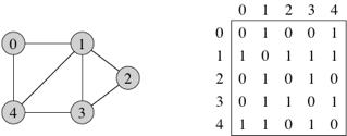
With an adjacency matrix, we can find out whether an edge is present in constant time, by just looking up the corresponding entry in the matrix. So what’s the disadvantage of an adjacency matrix? Two things, actually. First, it takes Θ(n2) space, even if the graph is sparse: relatively few edges. In other words, for a sparse graph, the adjacency matrix is mostly 0s, and we use lots of space to represent only a few edges. Second, if you want to find out which vertices are adjacent to a given vertex i, you have to look at all n entries in row i, taking Θ(n) time, even if only a small number of vertices are adjacent to vertex i.
For an undirected graph, the adjacency matrix is symmetric: the row i, column j entry is 1 if and only if the row j, column i entry is 1. For a directed graph, the adjacency matrix need not be symmetric.
Adjacency lists
Representing a graph with adjacency lists combines adjacency matrices with edge lists. For each vertex x, store a list of the vertices adjacent to it. We typically have a Python list of n adjacency lists, one adjacency list per vertex. We can store an adjacency list with a Python list (if we don’t plan to insert or delete adjacent vertices) or a linked list (if we expect to insert or delete adjacent vertices). Here’s an adjacency-list representation of the graph from above, using Python lists:
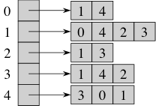
We can get to each vertex’s adjacency list in Θ(1) time, because we just have to index into a Python list of adjacency lists. To find out whether an edge (x,y) is present in the graph, we go to x’s adjacency list in Θ(1) time and then look for y in x’s adjacency list. How long does that take? O(d), where d is the degree of x, because that’s how long x’s adjacency list is. The degree of x could be as high as n − 1 (if x is adjacent to all other n − 1 vertices) or as low as 0 (if x is isolated, with no incident edges). In an undirected graph, y is in x’s adjacency list if and only if x is in y’s adjacency list. If the graph is weighted, then each item in each adjacency list is either a two-item list or a 2-tuple, giving the vertex number and the edge weight.
How much space do adjacency lists take? We have n lists, and although each list could have as many as n − 1 vertices, in total the adjacency lists for an undirected graph contain 2m items. Why 2m? Each edge (x,y) appears exactly twice in the adjacency lists, once in x’s list and once in y’s list, and there are m edges. For a directed graph, the adjacency lists contain a total of m items, one item per directed edge. For either an undirected graph or a directed graph, we say that the adjacency-list representation takes Θ(n+m) space; the n term comes from list of vertices, and the m term comes from all the adjacency lists together.
Adjacency lists in objects
For Lab Assignment 4, you’ll be creating several Vertex
objects. Among its instance variables, each Vertex object
will have one that is a reference to a Python list of
Vertex objects, indicating the adjacent vertices. There
will be two ways to get to a Vertex object: through the
adjacency list of some other Vertex object, or through a
dictionary whose keys are names of vertices and whose values are
Vertex objects.
Breadth-first search on a graph
One question we might ask about a graph is how few edges we need to traverse to find a path from one vertex to another. In other words, assuming that some path exists from vertex x to vertex y, find a path from x to y that has the fewest edges. You’ll be determining this quantity for a graph overlaid on the Dartmouth campus for Lab Assignment 4.
Another application is the famous Kevin Bacon game, which you program in CS 10. Consider a movie actor, say Renée Adorée, a silent film actress from the 1920s. She appeared in a film with Bessie Love, who made a movie with Eli Wallach, who acted in a film with Kevin Bacon, and so we say that Renée Adorée’s “Kevin Bacon number” is 3. If we were to make a graph where the vertices represent actors and we put an edge between vertices if their actors ever made a movie together, then we can use breadth-first search to find anyone’s Kevin Bacon number: the minimum number of actors between a given actor and Kevin Bacon.
Mathematicians have a similar concept, called an Erdős number. Paul Erdős was a great Hungarian mathematician. His Erdős number is 0. Mathematicians who coauthored a paper with Erdős have an Erdős number of 1. Mathematicians other than Erdős who coauthored a paper with those whose Erdős number is 1 have an Erdős number of 2. In general, a mathematician who coauthored a paper with someone whose Erdős number is k and did not coauthor a paper with anyone whose Erdős number is less than k has an Erdős number of k + 1. Believe it or not, there is even such a thing as an Erdős-Bacon number, which is the sum of the Erdős and Bacon numbers. A handful of people, including Erdős himself, have finite Erdős-Bacon numbers.
I’ll describe breadth-first search, which we abbreviate as BFS, for you, but I’ll give you no code. That’s because you’ll be implementing BFS in Lab Assignment 4.
We perform BFS from a given start vertex s. We can either designate a specific goal vertex, or we can just search to all vertices that are reachable from the start vertex (i.e., there exist paths from the start vertex to the vertices). We want to determine, for each vertex x that the search encounters, a shortest path from s to x, that is, a path from s to x with the minimum length (fewest edges).
We record two pieces of information about each vertex x:
The length of a shortest path from s to x, as the number of edges.
A backpointer from x, which is the vertex that immediately precedes x on a shortest path from s to x. For example, let’s look at that graph again:
In this graph, a shortest path from vertex D to vertex A is D, I, C, A, and so A would have a backpointer to C, C would have a backpointer to I, and I would have a backpointer to D. Because vertex D is the start vertex, no vertex precedes it, and so its backpointer is
None.This shortest path is not unique in this graph. Another shortest path from vertex D to vertex A is D, B, E, A. In this path, A would have a backpointer to E, E would have a backpointer to B, B would have a backpointer to D, and D’s backpointer would be
None.
I like to think of BFS in terms of sending waves of runners over the graph in discrete timesteps. We’ll focus on undirected graphs. I’ll call the start vertex s, and at first I won’t designate a goal vertex.
- Record the “distance” from the start vertex s to itself as 0, and record the
backpointer for s as
None. - At time 0, send out runners from s by sending out one runner over each edge incident on s. (So that the number of runners sent out at time 0 equals the degree of s.)
- Each runner arrives at a vertex adjacent to s at time 1. For each of these vertices, record its distance from s as 1 and its backpointer as s.
- At time 1, send out runners from each vertex whose distance from s is 1. As we did with s at time 0, send out one runner along each edge from each of these vertices.
- Each runner will arrive at another vertex at time 2. Let’s say that the runner left vertex x at time 1 and arrives at vertex y at time 2. Vertex y could have already been visited by a runner (perhaps it is s or perhaps it is another vertex that was visited at time 1). Or vertex y might not have been visited before. If vertex y had already been visited, forget about it; we already know its distance from s and its backpointer. But if vertex y had not already been visited, record its distance from s as 2, and record its backpointer as x (the vertex that the runner came from).
- At time 2, send out runners from each vertex whose distance from s is 2. As before, send out one runner along each edge from each of these vertices.
- Each runner will arrive at another vertex at time 3. If the vertex has been visited before, forget about it. Otherwise, record its distance from s as 3, and record its backpointer as the vertex from which the runner came.
- Continue in this way until all vertices that are reachable from the start vertex have been visited.
If there is a specific goal vertex, you can stop this process once it has been visited.
In the above graph, let’s designate vertex D as the start vertex, so
that D’s distance is 0 and its backpointer is None. At time
1, runners visit vertices G, B, and I, and so each of these vertices
gets a distance of 1 and D as their backpointers. At time 2, runners
from G, B, and I visit vertices D, G, B, I, F, E, C, and H. D, G, B, and
I have already been visited, but F, E, C, and H all get a distance of 2.
F and E get B as their backpointer, and C and H get I as their
backpointer. At time 3, runners from F, E, C, and H visit vertices B, A,
and I. B and I have already been visited, but A gets a distance of 3,
and its backpointer is set arbitrarily to either of E and C (it doesn’t
matter which, since either E or C precedes A on a shortest path from D).
Now all vertices have been visited, and the breadth-first search
terminates.
To determine the vertices on a shortest path, we use the backpointers
to get the vertices on a shortest path in reverse order. (But
you know how easy it is to reverse a list, and sometimes you’re fine
with knowing the path in reverse order, such as when you want to display
it.) Let’s look at the vertices on a shortest path from D to A. We know
that A is reachable from D because it has a backpointer. So A is on the
path, and it is preceded by its backpointer. Let’s say that A’s
backpointer is E (which I chose arbitrarily over C). So E is the next
vertex on the reversed path. E’s backpointer is B, and so B is the next
vertex on the reversed path. B’s backpointer is D, and so D is the next
vertex on the reversed path. D’s backpointer is None, and
so we are done constructing the reversed path: it contains, in order,
vertices A, E, B, and D.
Implementing BFS
You can’t implement BFS by following the above description exactly. That’s because you can’t send out lots of runners at exactly the same time. You can do only one thing at a time, and so you couldn’t send runners out along all edges incident on vertices G, B, and I all at the same time. You need to simulate doing that by sending out one runner at a time.
Let’s define the frontier of the BFS as the set of vertices that have been visited by runners but have yet to have runners leave them. If you send out runners one at a time, at any moment, the vertices in the frontier are all at either some distance i or distance i + 1 from the start vertex. For example, suppose that we have sent out runners from vertices D, G, and B so that they are no longer in the frontier. The frontier consists of vertex I, at distance 1, and vertices F and E, at distance 2.
One key to implementing BFS is to treat the frontier properly. In
particular, you want to maintain it in first in, first
out, or FIFO order. A data structure that
implements a FIFO order is called a queue. The
insert operation on a queue adds a new item, and the
delete operation removes the item that has been in the
queue for the longest time, returning the item.
Here is “pseudocode” (i.e., not real Python code) for BFS, where we maintain the frontier as as queue:
initialize the queue to contain only the start vertex s
distance of s = 0
while queue is not empty:
    x = queue.delete()   # remove vertex x from the queue
    for each vertex y that is adjacent to x:
        if y has not been visited yet:
            y's distance = x's distance + 1
            y's backpointer = x
            queue.insert(y)   # insert y into the queue
Now we have a few more questions to answer:
- How do we implement the queue?
- How do we represent the distance and backpointer for each vertex?
- How do we know whether a vertex has been visited?
Implementing a queue
It’s easy to implement a queue with a circular, doubly linked list with a sentinel. You should think about how you would do that.
It turns out that Python has a module called
collections, which implements various data structures. It
does not implement a queue, however. It implements something
even more general, called a deque, which is pronounced
like “deck” and means “double-ended queue.” If you think of a queue like
a line at Collis, where you enter at one end and leave at the other end,
a deque allows you to enter or leave at either end. So, of course, you
can use a deque as a queue by just inserting at one end and deleting at
the other, ignoring the functions (methods, actually) that allow you to
insert at the end you delete from and to delete at the end you insert
into. You’ll do just that in Lab Assignment 4. Read the instructions
carefully, because the methods you’ll be calling do not have
the names insert and delete.
Representing vertex information
Again, you have a couple of choices. If you create a class, say
Vertex, to represent what you need to know about a vertex,
it can have whatever instance variables you like. So a
Vertex object could have instance variables
distance, back_pointer, and even
visited. Of course, you could make visited
unnecessary by initializing distance to None
and saying that the vertex has been visited only if its
distance variable is not None (in which case
it would be the integer distance from the start vertex). Note that in
Lab Assignment 4, you won’t even need to keep track of distances.
This approach is nice because it encapsulates what you’d like to know
about a vertex within its object. But this approach has a downside: you
need to initialize the instance variables for every vertex
before you commence send out runners from the start vertex. You wouldn’t
want to use, say, the visited value from a previous BFS,
right? Ditto for the distance value.
There’s another way: use a dictionary. If you want to store
backpointers, store them in a dictionary, where the key is a reference
to a Vertex object and the value is a reference to the
Vertex object for its immediate predecessor on a shortest
path from the start vertex. You can use this same dictionary to record
whether a vertex has been visited, because you can say that a vertex has
been visited if and only if its Vertex object appears in
the dictionary. You can use the in operator to determine
whether the dictionary contains a reference to particular
Vertex object. The beauty of using a dictionary is that
initializing is E-Z: just make an empty dictionary. There is one other
detail you need to take care of: the start vertex. It has no
predecessor, but you want to record that it has been visited initially.
So you’ll need to store a reference to its Vertex object in
the dictionary, and you can just use None as the
corresponding value.